
X-ray transient classification for fun and profit, time reversal edition
Part three of many: a featurization baseline

One of the main limitations of traditional statistical learning methods, at least from the point of view of the practitioner, is that they need to be fed a data matrix with a fixed number of columns, known as features. This kind of tabular data is what standard statistical learning packages like scikit-learn usually take in input. Any piece of data that must be fed into such a pipeline has to be transformed into a fixed set of features: N numbers per data point. This is clearly both hard to do in a principled, unbiased way and suboptimal in terms of preserving information for data such as images or, as in our case, time series.
A strong appeal of deep learning is that it can make this featurization process largely automatic, as long as enough training data is available. In our case we have 806521 time series, which is certainly enough to train at least a small neural network. Still, deep learning features typically lack interpretability, and it is at any rate essential to establish a baseline with traditional methods to have a starting point against which to weight the pros and cons of deep learning.
One such approach I explored is the catch-22 set of time series features. Catch-22 features are a subset of the much larger pool of features known as HCTSA. HCTSA features capture a range of statistical and dynamical characteristics of time series, such as autocorrelation, entropy, periodicity, and stationarity. They are also a few thousands1, making them a pain to compute. Catch-22 solves this by selecting 22 features from HCTSA based on their performance on machine learning tasks on actual empirical data.
One of the most interesting among the Catch-22 features, at least from the point of view of a physicist is CO_trev_1_num (the original HCTSA name) or simply trev. Quoting from the Catch-22 manual:
trev computes the average across the time series of the cube of successive time-series differences. It will be close to zero for time series for which the distribution of successive decreases in the time series matches the distribution of successive increases, but will be positive if increases tend to be larger in magnitude and negative if decreases tend to be larger in magnitude.
This is closely related to the skewness of the distribution of increments of the time series. Under perfect time reversal symmetry one would expect the probability of any given positive increment moving from time t to t+1 to equal that of an equivalent negative increment. This would make the increment distribution symmetric and trev equal to zero, up to sampling error of course.
Interestingly, our time series yield values of trev ranging from roughly -40 to 40. This is how the histogram of our trev values looks like.
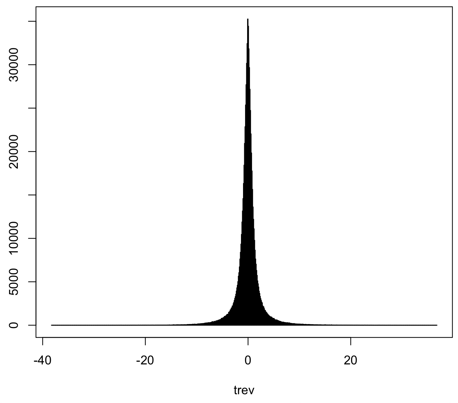
So while the individual light curve is not time-reversal symmetric, the overall distribution of trev, which can be taken to be a measure of symmetry violation, appears to be. But is it really?
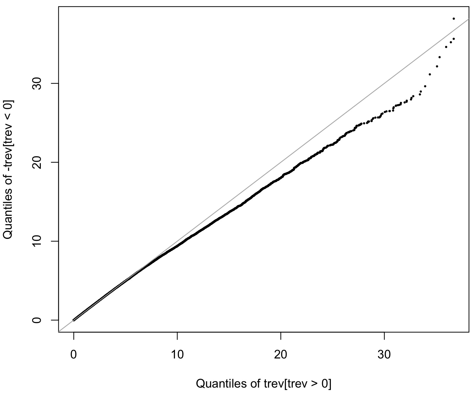
This one above is a quantile-quantile plot or Q-Q plot of the positive values of trev (the right side of the histogram in the previous plot) against minus the negative values of trev (the left side of the histogram, flipped). A Q-Q plot is a nice visual way to tell whether two samples come from the same distribution: just plot the quantiles of one sample against those of the other. If they align with the 1:1 line then the distributions match. This does not seem to be the case here, and as far as I can tell2 it is not a matter of a statistical fluctuation: there really seem to be more regions in the X-ray sky where time runs forwards than backwards.
4791 is the starting point of Lubba et al. 2019
By simulating time series made up of random, possibly autocorrelated, noise