Regression discontinuity and chaotic dynamics

Causation and real numbers

In a previous post I talked about regression discontinuity and how I introduced this statistical technique to astronomy. In an attempt to explain the concept, I simplified it as "we are using the least significant digits of the running variable as a random number generator". It turns out that this way to look at this technique is deeper than I thought.

First, let us recap with a concrete example: West Beirut and East Beirut were divided by the Green Line, a demarcation line that separated Muslims (West) and Christians (East) during the Lebanese civil war. An economist wants to know whether the treatment "being on the East side" has any lasting effect, say, on today's income. If you forget for the moment about the meandering nature of the line, you may model the problem as follows: longitude causes treatment by placing you either to the East or to the West of the line, and treatment causes outcome, via an unknown mechanism and possibly with vanishing intensity.

The Green Line, map credits to the CIA through Wikimedia commons.

So can you just compare East Beirut and West Beirut's outcomes by running some statistical test on the median income, get your p < 0.05 and call it a day? Unfortunately this would be too simplistic: longitude affects income also through other causal paths than just by placing you either to the East or to the West of the Green Line. For instance the distance to the sea, the elevation, the weather, the historical characteristics of the city (such as population density, building age, road quality, etc...) may all be affected by longitude and affect our outcome in turn. In other words, longitude is a confounding variable.

Regression discontinuity solves this by effectively breaking up longitude into two variables: a coarse-grained version of longitude, corresponding to the most significant digits of longitude -say two digits after the decimal point- and a residual corresponding to all the digits from the third one on. Martyr's square lies right on the Line, with a longitude of 35.507162, so this would yield a coarse-grained longitude of 35.50 and a residual of 0.007162(...). The assumption of regression discontinuity is that while the coarse grained longitude is confounded by all the factors listed above, the residual has an effect on the outcome of interest only through treatment, because confounding factors do not vary significantly on such a small scale. This translates to a directed acyclic graph as follows:

Directed acyclic graph for the regression discontinuity problem. See text for the meanings of the symbols. Own work.

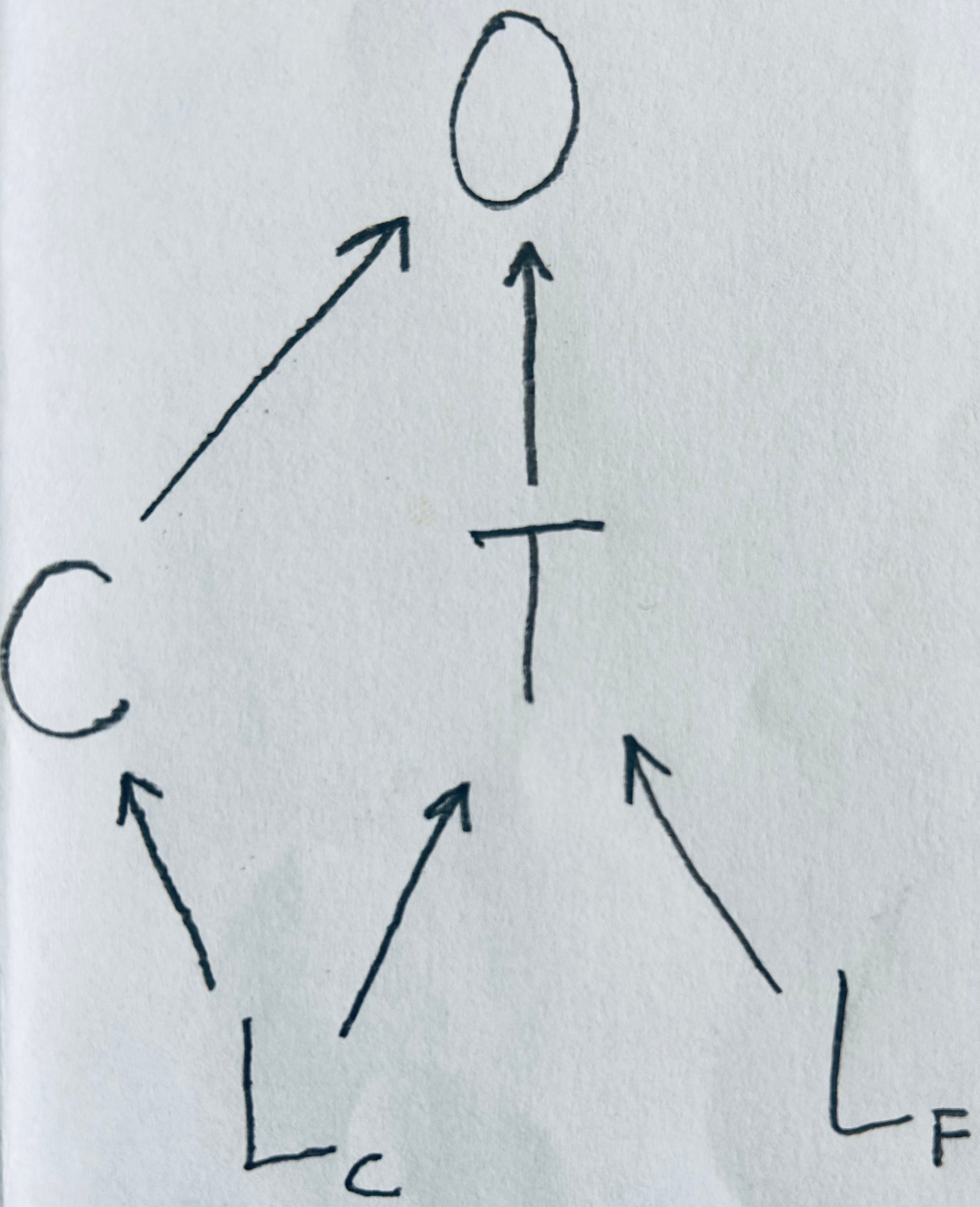
Here L_c stands for coarse longitude, L_f for fine longitude (the residual), T stands for treatment, O for outcome and C for other variables that mediate the confounding path through L_c between T and O. The backdoor criterion tells us that controlling for C would be enough to close this path, so that the resulting estimate of the causal effect of T on O would become unbiased. However we usually do not measure all the relevant Cs, so it is more convenient to control for L_c. We can do this because we preemptively separated L_c from L_f. In fact, we do not want to control for L_f (see Model 9 and Model 10 in A Crash Course in Good and Bad Controls). Alternatively, we could forget the backdoor criterion and just consider L_f as an instrumental variable: L_f causes O only through T.

This latter point of view is probably the most interesting. It also immediately raises a question: why are we confident that L_f is an instrumental variable? Why are digits that lie far to the right of the decimal point understood to lack causal parents, making them a good random number generator?

Here is where the nature of real numbers comes into play. Be warned: highly speculative stuff lies ahead. Whether you choose to make real numbers with Euclid-Dedekind cuts or with Cauchy sequences, they are not denumerable, per Cantor's diagonal argument. But algorithms are. So there is an infinity of non-computable real numbers. Not just that: computable reals have Lebesgue measure 0, which you could colorfully describe as basically any randomly chosen real number is going to be non computable¹.

An agent that relies on the identification of computable causal mechanisms to determine that a variable is caused by something -and thus is not (fully) random- will have to declare most real numbers random, that is not caused by anything.

This -minus the causal interpretation, which to the best of my knowledge is mine- has been discussed by Nicolas Gisin, for instance in Indeterminism in Physics, Classical Chaos and Bohmian Mechanics: are Real Numbers Really Real? and Real Numbers are the Hidden Variables of Classical Mechanics. He argues that so-called deterministic chaos is actually indeterministic, because as the chaotic evolution of a suitable system (such as the sawtooth map) reveals more and more digits of the system's initial conditions it is in fact creating those digits: they were not there to begin with, even though we usually assume that because we take initial conditions to be specified by real numbers, which are assumed known with infinite precision.

The connection with causality becomes clear if you look at whether you can find an instrumental variable in a physical system described by some Hamiltonian dynamics. If the system is integrable, the answer is no: once you switch to action-angle variables, all degrees of freedom end up evolving linearly with time, so everything perfectly correlates with everything else. There is no source of independent variation, no exogenous noise in structural causal model terminology. So no instrumental variables and no notion of causation. The coordinates and momenta of an integrable system are related to each other like X is related e.g. to X²: it does not sound meaningful to say that either causes the other. But this is not the case in a non-integrable system, which cannot be written in action-angle variables and can display chaos, that is the ability to amplify the least significant digits of its initial conditions.

Before reading Gisin's papers it was not clear to me that the integrable-chaotic divide was so fundamental, so I was having a hard time believing that it really had anything to do with our ability to model a dynamical system with Pearl's causality. I was not alone in this. Here I quote an email exchange I had with a colleague:

it seems to me that even if I have some *nonintegrable* systems, there will still be a perfect correlation in their behaviours over time. It is just that this correlation is much more difficult to describe. In other words, I don’t think the line between `logical connection’² and ‘causal connection’ is drawn between integrable and nonintegrable systems.

His argument here is that a chaotic flow is still a deterministic map on phase space. Every degree of freedom at time t is still a function of the initial conditions. The correlation among different coordinates remains perfect, just more complicated. This argument falls apart if we admit, with Gisin, that chaotic dynamics is not merely deterministically revealing more and more digits past the decimal points in our initial conditions, but is instead creating those digits as time goes by, making them genuinely random. It is this genuine randomness -the same randomness leveraged by regression discontinuity³- that makes instrumental variables (or exogenous noises) possible.

1. When we actually do physics, all the numbers we use are by necessity computable, so real numbers are a glaring violation of Occam's razor. We mostly just don’t care.

2. In the context of our conversation “logical connection” meant the kind of relation between X and X squared, to which we cannot assign a clear causal meaning.

3. Interestingly, the basic setup of regression discontinuity requires treatment to be a step function of the running variable. If treatment has any effect, this yields a sensitive dependence on initial conditions at least in the neighborhood of the threshold.